From the Panopticon has migrated to its new Wordpress home. Currently finding inspiration to put the message of the images to words.
*needs another bump from the tricycle.
Thursday, September 23, 2010
Tuesday, August 3, 2010
Migrating very soon
There have been no updates recently because of the impending migration of this blog. It will be posted here when its up and ready. The entries published here will be migrated with edited content.
This account will not be deleted.
This account will not be deleted.
Thursday, July 8, 2010
The Crab Decomposition
work in progress
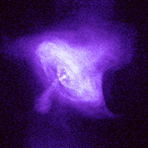
Last January Doc Muriel discussed something about laminar fluids emitting blue light and that turbulent fluids would emit at a lower wavelength. He showed a picture of the Crab Nebula and the decomposition to blue. The result showed a blue ring at the center of the Nebula. It surprised me that such phenomena as laminar fluids in space could be seen in a simple nebula image. I never saw it again.
I'd love to have a 7-band image of the nebula; all I have so far is a snapshot from Stellarium. I tried to get the blue channel. Of course it's an RGB image and the blue channel also contributes to form other colors.
Here is an attempt to further filter the blue channel by removing pixels that overlap higher level red and green (>0.7 with max 1.0). It's a crude attempt but I'll build on this and find an actual decomposition of the nebula for comparison.

the Crab Nebula taken from Stellarium

blue channel

result of filtering out the other colors
Here are nice crab photos
Here is the code.
A =imread('crab.png');
red = A(:,:,1);
green = A(:,:,2);
blue = A(:,:,3);
//red channel
R = A;
R(:,:,2) = 0;
R(:,:,3) = 0;
//green channel
G = A;
G(:,:,1) = 0;
G(:,:,3) = 0;
//blue channel
B = A;
B(:,:,1) = 0;
B(:,:,2) = 0;
scf(2); imshow(B)
scf(3); imshow(B(:,:,3));
//640-490nm
rc = R(:,:,1);
rc(find(rc>0.7)) = 0;
gc = G(:,:,2);
gc(find(gc>0.7)) = 0;
blue = B(:,:,3).*rc.*gc;
B(:,:,3) = blue;
scf(4);imshow(blue);
imwrite(blue, 'bluecrab.png');
imwrite(B(:,:,3), 'bluechannel.png');
imwrite(B, 'bluecrab3.png');
Last January Doc Muriel discussed something about laminar fluids emitting blue light and that turbulent fluids would emit at a lower wavelength. He showed a picture of the Crab Nebula and the decomposition to blue. The result showed a blue ring at the center of the Nebula. It surprised me that such phenomena as laminar fluids in space could be seen in a simple nebula image. I never saw it again.
I'd love to have a 7-band image of the nebula; all I have so far is a snapshot from Stellarium. I tried to get the blue channel. Of course it's an RGB image and the blue channel also contributes to form other colors.
Here is an attempt to further filter the blue channel by removing pixels that overlap higher level red and green (>0.7 with max 1.0). It's a crude attempt but I'll build on this and find an actual decomposition of the nebula for comparison.

the Crab Nebula taken from Stellarium

blue channel

result of filtering out the other colors
Here are nice crab photos
x-rays from Crab Nebula
Here is the code.
A =imread('crab.png');
red = A(:,:,1);
green = A(:,:,2);
blue = A(:,:,3);
//red channel
R = A;
R(:,:,2) = 0;
R(:,:,3) = 0;
//green channel
G = A;
G(:,:,1) = 0;
G(:,:,3) = 0;
//blue channel
B = A;
B(:,:,1) = 0;
B(:,:,2) = 0;
scf(2); imshow(B)
scf(3); imshow(B(:,:,3));
//640-490nm
rc = R(:,:,1);
rc(find(rc>0.7)) = 0;
gc = G(:,:,2);
gc(find(gc>0.7)) = 0;
blue = B(:,:,3).*rc.*gc;
B(:,:,3) = blue;
scf(4);imshow(blue);
imwrite(blue, 'bluecrab.png');
imwrite(B(:,:,3), 'bluechannel.png');
imwrite(B, 'bluecrab3.png');
Tuesday, July 6, 2010
FOSSY Things: Histogram Equalization
Image contrast is changed by manipulating the PDF of the image. One can easily use popular image processing software like Photoshop and GIMP to achieve similar results. Inkscape, a vector-graphics software can also do the same thing. The software is a parallel of Illustrator. It is specialized for creating vectors but can also import raster graphics and do a variety of enhancements.
Here is a sample of some Inkscape tricks. The image used here was created with TuxPaint, a FOSS kiddie version of Photoshop and Paint.
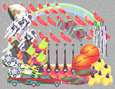
Image created from TuxPaint with the Stamps extension
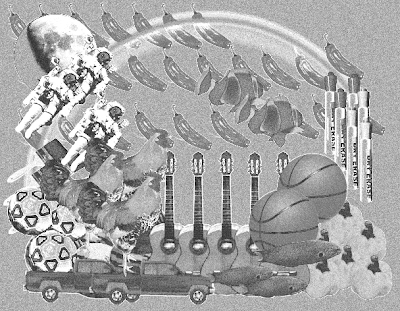
Here is a grayscale version of the image
Conversion was done with GIMP 2.6
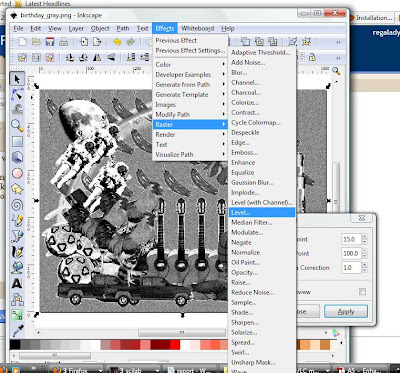
The gray and white points can be edited with the Raster>Level feature in Inkscape 0.46
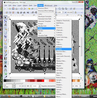
Equalize does the same trick but it doesn't have customizable settings
Here is a sample of some Inkscape tricks. The image used here was created with TuxPaint, a FOSS kiddie version of Photoshop and Paint.

Image created from TuxPaint with the Stamps extension

Here is a grayscale version of the image
Conversion was done with GIMP 2.6
You can't really manipulate the CDF curves like what we did in the previous post but it can do the same trick. With Levels, you simply change white and black points, like having a threshold for both black and white. I assume that Equalize performs a histogram equalization. For the curious, Inkscape effects are written in Python and codes can be viewed after installation.

The gray and white points can be edited with the Raster>Level feature in Inkscape 0.46

Equalize does the same trick but it doesn't have customizable settings
Using GIMP, one can manipulate the CDF by hand and see the PDF change live.
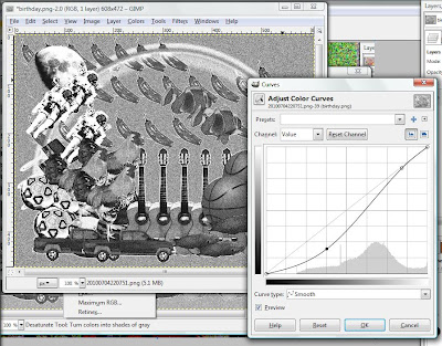
Colors>Curves trick from GIMP 2.6

Colors>Curves trick from GIMP 2.6
Here are the final images.

Enhanced with Inkscape's Equalize

Enhanced with Inkscape's Level

Enhanced with GIMP's Curves
Inkscape, GIMP and TuxPaint are Free and Open Source and can be easily downloaded over the internet. Thanks to Leon of CPU and Last Year's Software Freedom Day for the OpenEduDisc. I stumbled upon TuxPaint on that disc in search for graphics software goodies.
Many thanks to Shugo Tokumaru and Lost in Found for making beautiful music to keep me company.

Enhanced with Inkscape's Equalize

Enhanced with Inkscape's Level

Enhanced with GIMP's Curves
Many thanks to Shugo Tokumaru and Lost in Found for making beautiful music to keep me company.
Saturday, July 3, 2010
5. Enhancement by Histogram Manipulation
In the previous post on image types and formats, I used the histogram of a grayscale image to select the threshold for binary conversion. The histogram gives the distribution of pixels over various graytones or levels (PDF, Probability Distribution Function when normalized). Image enhancement can be done by manipulating the PDF of an image.


The original image with poor contrast and image enhanced by linear backprojection of the CDF
To increase the contrast of images, the pixels must be distributed over a wide range of gray levels. Histogram manipulation can be accomplished by using the CDF (Cumulative Distribution Function). The CDF is described by the following equation,

A linear CDF would then do the trick of increasing PDF spread. Having CDF values plotted against itself would yield a linear plot. Each pixel must then take on its corresponding CDF value as its new gray level.
Notice that in the new PDF, pixels distribution are more spread especially at the 0-0.6 region. The old PDF is in 0-255 format since this is the default configuration of the imwrite() function. The new PDF is in 0-1.0 formats because it was taken from normalized values of the old CDF.
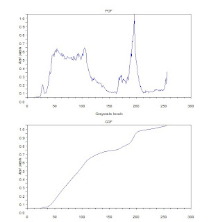
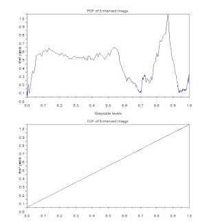
PDF and CDF of original image (left) and the enhance image (right)
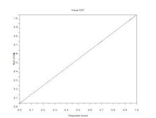
linear CDF as reference for backprojection
Aside from a linear CDF, a simple matrix manipulation can create a nonlinear CDF. A logarithmic CDF (y = log(x)) was applied. CDF values do not change in the white end of the scale and more pixels are concentrated in the dark region. Consequently, the result is a low contrast, dark image.

Image enhanced by a logarithmic CDF

PDF and CDF of image with logarithmic enhancement
Since I used histplot() on the last activity, I was fixated on how to access the values from histplot(). Histplot uses dsearch() which in turn makes use of tabul(). Thanks to the excellent Scilab Help modules. A simple use of find() by Gilbert Gubatan accomplishes the same thing. The difference with the latter is that tabul() does not store values for empty classes. In the case of the featured image, the length of the array is equal to 244 instead of 256. It is necessary to consider this in backprojection. Intuitively, one would index the CDF values with 0:255, which will not work for a 244 long array. See the code below.
Special thanks to Carmen Lumban who took the photo in 2008.
I give myself a 10/10 for this activity.
Code
A =imread('e_gray.jpg');
Amax = max(A);
Amin = min(A);
//get PDF of original image
p = tabul(A,'i');
scf(0); subplot(211);
plot(p(:,1),p(:,2)/max(p(:,2)));
title('PDF');
xlabel('Grayscale levels');
ylabel('# of pixels');
//get CDF of original image
c0 = cumsum(p(:,2)); //2nd col of p
c = c0/max(c0);
scf(0); subplot(212);
plot(p(:,1),c);
title('CDF')
xlabel('Grayscale levels');
ylabel('# of pixels');
//plot uniformly distributed CDF
x = c;
scf(1);
plot(x,x);
title('linear CDF');
xlabel('Grayscale levels');
ylabel('# of pixels');
//backplot uniform CDF to image
B = []; //enhanced image matrix
i = 0;
j = 0;
k= 0;
for i = 1:size(A,1)
for j = 1:size(A,2)
k = find(p(:,1)==A(i,j));
B(i,j) = c(k);
end
end
//get new PDF
p2 = tabul(B,'i');
scf(2); subplot(211);
plot(p2(:,1),p2(:,2)/max(p2(:,2)));
title('PDF of Enhanced Image');
xlabel('Grayscale levels');
ylabel('# of pixels');
//get new CDF
c02 = cumsum(p2(:,2)); //2nd col of p
c2 = c02/max(c02);
scf(2); subplot(212);
plot2d(p2(:,1),c2);
title('CDF of Enhanced Image');
xlabel('Grayscale levels');
ylabel('# of pixels');
C = []; //enhanced image, log
i = 0;
j = 0;
k= 0;
clog0 = abs(log(c));
clog = clog0/max(clog0);
for i = 1:size(A,1)
for j = 1:size(A,2)
k = find(p(:,1)==A(i,j));
C(i,j) = clog(k);
end
end
//get PDF of new image
p3 = tabul(C,'i');
scf(3); subplot(211);
plot(p3(:,1),p3(:,2)/max(p3(:,2)));
title('PDF of Enhanced Image: Logarithmic CDF');
xlabel('Grayscale levels');
ylabel('# of pixels');
//get new CDF
c03 = cumsum(p2(:,2)); //2nd col of p
c3 = c03/max(c03);
scf(3); subplot(212);
plot2d(p3(:,1),c3);
title('CDF of Enhanced Image: Logarithmc CDF');
xlabel('Grayscale levels');
ylabel('# of pixels');
imwrite(B, 'C:\Users\regaladys\Desktop\e_gray2.jpg');
imwrite(C, 'C:\Users\regaladys\Desktop\elog_gray2.jpg');
Definition of the Cumulative Distribution Function
A linear CDF would then do the trick of increasing PDF spread. Having CDF values plotted against itself would yield a linear plot. Each pixel must then take on its corresponding CDF value as its new gray level.
Notice that in the new PDF, pixels distribution are more spread especially at the 0-0.6 region. The old PDF is in 0-255 format since this is the default configuration of the imwrite() function. The new PDF is in 0-1.0 formats because it was taken from normalized values of the old CDF.


PDF and CDF of original image (left) and the enhance image (right)

linear CDF as reference for backprojection

Image enhanced by a logarithmic CDF

PDF and CDF of image with logarithmic enhancement
Since I used histplot() on the last activity, I was fixated on how to access the values from histplot(). Histplot uses dsearch() which in turn makes use of tabul(). Thanks to the excellent Scilab Help modules. A simple use of find() by Gilbert Gubatan accomplishes the same thing. The difference with the latter is that tabul() does not store values for empty classes. In the case of the featured image, the length of the array is equal to 244 instead of 256. It is necessary to consider this in backprojection. Intuitively, one would index the CDF values with 0:255, which will not work for a 244 long array. See the code below.
Special thanks to Carmen Lumban who took the photo in 2008.
I give myself a 10/10 for this activity.
Code
A =imread('e_gray.jpg');
Amax = max(A);
Amin = min(A);
//get PDF of original image
p = tabul(A,'i');
scf(0); subplot(211);
plot(p(:,1),p(:,2)/max(p(:,2)));
title('PDF');
xlabel('Grayscale levels');
ylabel('# of pixels');
//get CDF of original image
c0 = cumsum(p(:,2)); //2nd col of p
c = c0/max(c0);
scf(0); subplot(212);
plot(p(:,1),c);
title('CDF')
xlabel('Grayscale levels');
ylabel('# of pixels');
//plot uniformly distributed CDF
x = c;
scf(1);
plot(x,x);
title('linear CDF');
xlabel('Grayscale levels');
ylabel('# of pixels');
//backplot uniform CDF to image
B = []; //enhanced image matrix
i = 0;
j = 0;
k= 0;
for i = 1:size(A,1)
for j = 1:size(A,2)
k = find(p(:,1)==A(i,j));
B(i,j) = c(k);
end
end
//get new PDF
p2 = tabul(B,'i');
scf(2); subplot(211);
plot(p2(:,1),p2(:,2)/max(p2(:,2)));
title('PDF of Enhanced Image');
xlabel('Grayscale levels');
ylabel('# of pixels');
//get new CDF
c02 = cumsum(p2(:,2)); //2nd col of p
c2 = c02/max(c02);
scf(2); subplot(212);
plot2d(p2(:,1),c2);
title('CDF of Enhanced Image');
xlabel('Grayscale levels');
ylabel('# of pixels');
C = []; //enhanced image, log
i = 0;
j = 0;
k= 0;
clog0 = abs(log(c));
clog = clog0/max(clog0);
for i = 1:size(A,1)
for j = 1:size(A,2)
k = find(p(:,1)==A(i,j));
C(i,j) = clog(k);
end
end
//get PDF of new image
p3 = tabul(C,'i');
scf(3); subplot(211);
plot(p3(:,1),p3(:,2)/max(p3(:,2)));
title('PDF of Enhanced Image: Logarithmic CDF');
xlabel('Grayscale levels');
ylabel('# of pixels');
//get new CDF
c03 = cumsum(p2(:,2)); //2nd col of p
c3 = c03/max(c03);
scf(3); subplot(212);
plot2d(p3(:,1),c3);
title('CDF of Enhanced Image: Logarithmc CDF');
xlabel('Grayscale levels');
ylabel('# of pixels');
imwrite(B, 'C:\Users\regaladys\Desktop\e_gray2.jpg');
imwrite(C, 'C:\Users\regaladys\Desktop\elog_gray2.jpg');
4. Area Estimation for Images with Defined Edges
With Green's Theorem one can easily calculate the area of images. This requires defined edges and Scilab with the SIP Toolbox accomplishes edge detection with follow().
Img = imread('circle.bmp');
[x,y] = follow(Img);
plot2d(x,y, rect = [0,0,200,200]);
l = length(x);
area = 0;
area_updated = 0;
for i=1:l-1
area_add = (x(i)*y(i+1)) - (x(i+1)* y(i));
area_updated = area_updated + area_add;
end
area = area_updated/2;
plot2d() displays the edges of the image defined in matrix [x,y]. Area is calculated in terms of pixels. The analytic value of the area is the number of pixels defining the image. With a white image, each matrix element is of the value 1. The area is simply given by sum(). Accuracy of the measurement is calculated by taking the difference of calculated area and the analytic value.
area_pixel= sum(Img);
dif = area - area_pixel;
area_acc = abs(dif*100/area_pixel);
Using synthetic images generated with Scilab, I calculated their areas with Green's Theorem.


With the available satellite images of Wikimapia, I was able to take images of the subdivision where we live in Bacolod City.
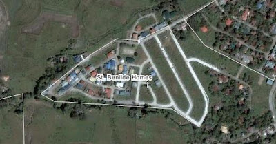
Satellite image of St. Benilde Homes, Mansilingan City
It appears to be taken before 2006
photo courtesy of Wikimapia

Img = imread('circle.bmp');
[x,y] = follow(Img);
plot2d(x,y, rect = [0,0,200,200]);
l = length(x);
area = 0;
area_updated = 0;
for i=1:l-1
area_add = (x(i)*y(i+1)) - (x(i+1)* y(i));
area_updated = area_updated + area_add;
end
area = area_updated/2;
plot2d() displays the edges of the image defined in matrix [x,y]. Area is calculated in terms of pixels. The analytic value of the area is the number of pixels defining the image. With a white image, each matrix element is of the value 1. The area is simply given by sum(). Accuracy of the measurement is calculated by taking the difference of calculated area and the analytic value.
area_pixel= sum(Img);
dif = area - area_pixel;
area_acc = abs(dif*100/area_pixel);
Using synthetic images generated with Scilab, I calculated their areas with Green's Theorem.


Synthetic images with calculated areas of up to 97.8% and 97.3% accuracy

With the available satellite images of Wikimapia, I was able to take images of the subdivision where we live in Bacolod City.

Satellite image of St. Benilde Homes, Mansilingan City
It appears to be taken before 2006
photo courtesy of Wikimapia

Zooming in on Block 5, the Regalado Residence is indicated by the cross marking
photo courtesy of Wikimapia
photo courtesy of Wikimapia
I intend to calculate the total area of the subdivision and Block 5. To create solid bw images of these photos I used GIMP 2.6. I used the free select tool to create a mask of the block's shape and filled a white layer with black.

Black and white bitmap file of Block 5 for image detection and area estimation
With the map's scale, the conversion is approximately 5.25 m/pixel. This is calculated with the method described in Activity 1.
The area was calculated to 95.6% accuracy with the block measuring up to 11,103 square meters by area estimation and 11,620 square meters as the analytic value.
Here is the full code used to calculate the Block 5 area. Note that the bitmap file is a truecolor image though it appears to be in black and white. It must be first converted to a binary image before area estimation. Without this step, follow() function will not detect images as the truecolor file will have 3 channels for RGB, not compatible for the operation of follow().
//area estimation by green's function
Img = gray_imread('block5_w2.bmp');
histplot([0 : 0.05 : 1.0], Img)
Img2 = im2bw(Img, 0.5);
[x,y] = follow(Img2);
plot2d(x,y, rect = [0,0,200,200]);
l = length(x);
area = 0;
area_updated = 0;
for i=1:l-1
area_add = (x(i)*y(i+1)) - (x(i+1)* y(i));
area_updated = area_updated + area_add;
end
area = area_updated/2;
area_pixel= sum(Img);
dif = area - area_pixel;
area_acc = 100 - abs(dif*100/area_pixel);
Thanks to Ricardo Fabri, author of most of SIP, for keeping beautiful and simple docstrings on his macros. It took me a while to realize that the .bmp file must be converted to a binary image. Nevertheless, I have completed this exercise with more ease than the previous two. I feel a considerable improvement in my familiarity with Scilab and SIP.
For this activity I give myself a 10/10. I think this entry has achieved a simpler format in comparison to the previous discussions. Thanks to "Mother Earth" (mom) for reading this blog and telling me that she cannot understand anything. It has compelled me to write simpler and I hope to post more entries in the future.
Wednesday, June 30, 2010
3. Image Types and Formats
There are two classifications of computer graphics according to how the image is formed. (1) Raster graphics or bitmaps define images pixel-by-pixel, (2) and Vector graphics that store images as paths or mathematical relations of points. Most font formats are stored as vectors to retain optimum resolution at various sizes. These images are then easily converted to bitmaps.
Lately I've been fascinated by these open-source graphics softwares - GIMP, Inkscape and Blender. GIMP is a raster graphics software similar to PhotoShop. Everyone in class is familiar with it when we used it an optics class last year. Inkscape on the other-hand is a vector graphics software. Best used with a tablet, Inkscape creations can be easily resized to whatever resolution (dpi) or dimension (pixel dimensions). Images are stored in Scalable Vector Graphics Format (.svg).
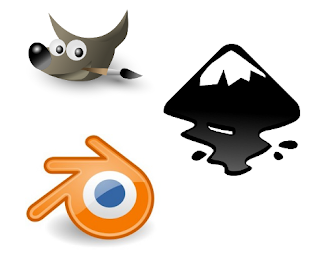 Blender differs from these two as a 3-D graphics and animation software. Objects are created using vectors and can be texturized by raster graphics. Last year's Software Freedom Day boasted a talk on Blender by no one else than the young artist of Pinoy Blender Users' Group (PBUG). They use GIMP to create textures. Blender conforms these flat, two-dimensional images along the contour of 3D objects. A GIMP enthusiast also shared how contributors can custom-code a request for special filters or effects (posted up for the public in .py files).
 Binary Image courtesy of NASA
http://idlastro.gsfc.nasa.gov/idl_html_help/images/imgdisp01.gif
 Grayscale Image courtesy of NASA
http://idlastro.gsfc.nasa.gov/idl_html_help/images/imgdisp02.gif
 Truecolor Image of jaguar fur
courtesy of National Geographic
Size: 150x200

 Truecolor and grayscale conversion done with Scilab
 Graytones of the converted pixel art image
Lately I've been fascinated by these open-source graphics softwares - GIMP, Inkscape and Blender. GIMP is a raster graphics software similar to PhotoShop. Everyone in class is familiar with it when we used it an optics class last year. Inkscape on the other-hand is a vector graphics software. Best used with a tablet, Inkscape creations can be easily resized to whatever resolution (dpi) or dimension (pixel dimensions). Images are stored in Scalable Vector Graphics Format (.svg).
The prospect of coding my own filter and effects is something I look forward to as the lessons in this course progress. But before we proceed to the meaty codes ahead, here is a review of different image types and formats.According to the color or how color is mapped, digitized images can be categorized into 4 basic categories.
Binary Images, each pixel is either a black or a white and is represented by ones and zeros.
Binary Image courtesy of NASA http://idlastro.gsfc.nasa.gov/idl_html_help/images/imgdisp01.gif
Size: 362x362
File Size: 5135
Format: GIF
Depth: 8
Storage Type: Indexed
Number of Colors: 256
Resolution Unit: centimeter
XResolution: 72
YResolution: 72
Grayscale images, each pixel has a value between white (255) and black (0). Color is limited to graytones. The following image is taken from NASA
Format: GIF
Depth: 8
Storage Type: Indexed
Number of Colors: 256
Resolution Unit: centimeter
XResolution: 72
YResolution: 72
Grayscale images, each pixel has a value between white (255) and black (0). Color is limited to graytones. The following image is taken from NASA
Grayscale Image courtesy of NASA http://idlastro.gsfc.nasa.gov/idl_html_help/images/imgdisp02.gif
Size: 248x248
File Size: 10369
Format: GIFDepth: 8
Storage Type: Indexed
Number of Colors: 8
XResolution: 72.0
YResolution: 72.0
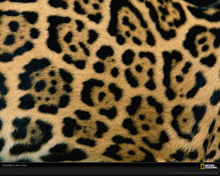
Truecolor images, the image is composed of channels in red, green and blue. The color of each pixel is determined by the superposition of each channel. The following jaguar fur is a sample of a trucolor image. Note on the image information that the number of colors is zero. Given that this is a truecolor image, it does not store an index of colors, hence the zero number of colors indicated.
File Size: 10369
Format: GIFDepth: 8
Storage Type: Indexed
Number of Colors: 8
XResolution: 72.0
YResolution: 72.0
Truecolor images, the image is composed of channels in red, green and blue. The color of each pixel is determined by the superposition of each channel. The following jaguar fur is a sample of a trucolor image. Note on the image information that the number of colors is zero. Given that this is a truecolor image, it does not store an index of colors, hence the zero number of colors indicated.
 Truecolor Image of jaguar fur
courtesy of National Geographic
Size: 1280x1024
File Size: 357929
Format: JPEG
Depth: 8
Storage Type: Truecolor
Number of Colors: 0
XResolution: 100.0
YResolution: 100.0
File Size: 357929
Format: JPEG
Depth: 8
Storage Type: Truecolor
Number of Colors: 0
XResolution: 100.0
YResolution: 100.0
Indexed Images differ from truecolor in that color information is compressed into a single index of colors. This allows compression of an image to a smaller file size.
 indexed image
http://upload.wikimedia.org/wikipedia/en/7/7c/Adaptative_8bits_palette_sample_image.png indexed image
Size: 150x200
File Size: 25575
Format: PNG
Depth: 8
Storage Type: Indexed
Number of Colors: 256
XResolution: 72
YResolution: 72
Format: PNG
Depth: 8
Storage Type: Indexed
Number of Colors: 256
XResolution: 72
YResolution: 72
Advanced Image Types
With the expansion of imaging to fields like medicine and astronomy, advanced image types have surfaced. Here are some examples of advanced image types.
Multispectral images scan every pixel at different bands. For the Landsat, topographical images are taken up to 7 bands (3 for RGB and 4 for various IR bands). Information can be used for coastal area mapping, differentiating vegetation and snows from clouds among other meteorological applications. Hyperspectral images on the other hand take images from IR to visible and UV. One can imagine having the spectra of each pixel.
 Southeastern Indonesia
Taken by Landsat
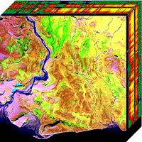 Hyperspectral cube, plane seen here is the visible spectra information, the sides of the cube are the edges of images taken in UV and IR bands. Photo taken by NASA
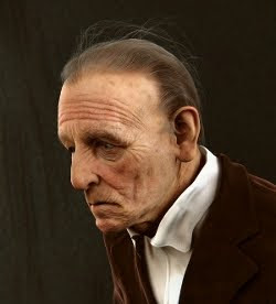 Image taken by setting up a virtual camera and lighting to take a picture of a 3D old man
Blender rendered by Kamil Mikawski
File Formats
Various image types differ on the kind of information stored recording images. These information can be stored or compressed in various file formats. Wikipedia gives a rundown of standard file formats. It surprised me that wiki documented 233 different file formats in existence. Formats like EMF (enhanced metafile) and SGB are supported only by Microsoft and Sun Microsystems respectively for their own software. There are also patented formats (HD Photo by Microsoft), and those created for Mars Rovers (ICER).
The most common image formats however, are TIF, BMP, GIF, PNG and JPEG.
BMP (bitmap) - 1 to 32-bit color depth/ supports transparencies and indexed color
GIF (Graphics Interchange Format) - 1 to 8-bit color depth/ support indexed color, transparencies, layers and animation/
JPEG (Joint Photographic Experts Group) - 8, 12, 24-bit color depth
PNG (Portable Network Graphics) - 1, 2, 4, 8, 16, 24, 32, 48, 64-bit color depth/ supports transparencies and indexed color
TIFF (Tagged Image File Format) - 1, 2, 4, 8, 16, 24, 32-bit color depth/ supports indexed color, transparencies and layers
Color depth refers to the representation of each pixel in bits.
Compression of these formats can either be lossy or lossless. In lossless, the original can be reconstructed from the compression. PNG and GIF use lossless compression while TIFF and JPEG can use lossy compression. This is also the same for other file formats.
With the expansion of imaging to fields like medicine and astronomy, advanced image types have surfaced. Here are some examples of advanced image types.
Multispectral images scan every pixel at different bands. For the Landsat, topographical images are taken up to 7 bands (3 for RGB and 4 for various IR bands). Information can be used for coastal area mapping, differentiating vegetation and snows from clouds among other meteorological applications. Hyperspectral images on the other hand take images from IR to visible and UV. One can imagine having the spectra of each pixel.
Southeastern IndonesiaTaken by Landsat
 Hyperspectral cube, plane seen here is the visible spectra information, the sides of the cube are the edges of images taken in UV and IR bands. Photo taken by NASA
 Image taken by setting up a virtual camera and lighting to take a picture of a 3D old man
 Blender rendered by Kamil Mikawski
File Formats
Various image types differ on the kind of information stored recording images. These information can be stored or compressed in various file formats. Wikipedia gives a rundown of standard file formats. It surprised me that wiki documented 233 different file formats in existence. Formats like EMF (enhanced metafile) and SGB are supported only by Microsoft and Sun Microsystems respectively for their own software. There are also patented formats (HD Photo by Microsoft), and those created for Mars Rovers (ICER).
The most common image formats however, are TIF, BMP, GIF, PNG and JPEG.
BMP (bitmap) - 1 to 32-bit color depth/ supports transparencies and indexed color
GIF (Graphics Interchange Format) - 1 to 8-bit color depth/ support indexed color, transparencies, layers and animation/
JPEG (Joint Photographic Experts Group) - 8, 12, 24-bit color depth
PNG (Portable Network Graphics) - 1, 2, 4, 8, 16, 24, 32, 48, 64-bit color depth/ supports transparencies and indexed color
TIFF (Tagged Image File Format) - 1, 2, 4, 8, 16, 24, 32-bit color depth/ supports indexed color, transparencies and layers
Color depth refers to the representation of each pixel in bits.
Compression of these formats can either be lossy or lossless. In lossless, the original can be reconstructed from the compression. PNG and GIF use lossless compression while TIFF and JPEG can use lossy compression. This is also the same for other file formats.
Grayscale images, treshold and conversion
RGB images are easily converted to grayscale with scilab's SIP toolbox functions im2gray and gray_imread.
Last week, I tried using Inkscape to practice making pixel art, an art form making it's comeback from the 80s. Here is a sample of three spaceship/hearts in different colors. Using the following code, the image was read and converted to grayscale,
Img = gray_imread('5.jpg');
histplot([0:0.05:1.0], Img)
imwrite(Img, 'C:\Users\regaladys\Desktop\5_gray.jpg');
histplot([0:0.05:1.0], Img)
imwrite(Img, 'C:\Users\regaladys\Desktop\5_gray.jpg');


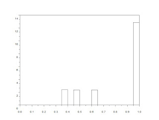
A histogram then displays the distribution of the pixels over different graylevels (Probability Distribution Function or PDF). Those at the 0 end are the darker pixels and a level of 1.0 means the pixel is white. Graylevel values are from 0 to 255 and is normalized by the histplot function.
Graytones of the converted pixel art imageThe histogram is useful in determining the threshold level for binary conversion. Values over the threshold level are converted to white and lower values are converted to black. Adjusting the treshold level can remove a lighter background or unwanted elements in the image.
The PDF information of the pixelships shows pixel concentrations at 1.0 and three other gray-levels. Binary conversion at different threshold values can remove one of the pixelships. Binary conversion of a grayscale is executed in a line of code.
Img=im2bw('5_gray.jpg', 0.8);
imwrite(Img, 'C:\Users\regaladys\Desktop\5_black1.jpg');

threshold at 0.8

threshold at 0.6

threshold at 0.45
Another example is Nat Geo's jaguar fur wallpaper. With a more diverse range of shades and hues, the PDF of this image is more spread. In binary conversion of the image, I wanted to isolate the jaguar's spots. This requires a threshold of around 0.25.


During conversion, image dimensions (matrix size) were not changed. But with lower amounts of color information, file sizes decrease after grayscale and binary conversion (312 KB for the truecolor image, 39.6 KB and 54.3 KB for the grayscale and binary conversions).
Binary conversion is also useful in cleaning up grayscale text scans. Here is Activity 1's plot taken from an old journal and the clean-up by binary conversion.
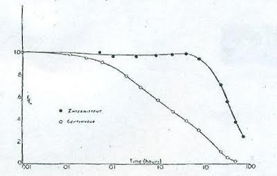
Scanned scientific plot from an old journal
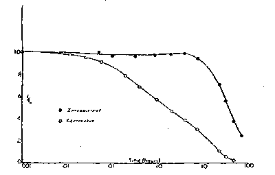
Binary version of the scanned plot removes the unwanted background color
For this activity I give myself a 9/10. Most of the difficulty in the activity was encountered during the image conversion. Also writing and editing take up more time than the actual research. This blog though is an exercise to write the next blog entries more efficiently. It was fun creating the entries but it can also become a form of distraction from coursework. Making these entries are so addicting. hehehe.
On the more technical side, one must remember to increase stacksize and use images with smaller dimensions.
I would like to thank wifi hotspots, Mushroomburger and McDonalds in Katipunan that housed me for several nights to complete the activities.
References
Scilab 4.1.2 Documentation
M. Soriano. A3 - Image Types and Formats. NIP, University of the Philippines. 2010.
Remote Sensing Tutorial. NASA. http://rst.gsfc.nasa.gov/
Geoscience Australia. http://www.ga.gov.au/
www.blender.org
www.wikipedia.com
The PDF information of the pixelships shows pixel concentrations at 1.0 and three other gray-levels. Binary conversion at different threshold values can remove one of the pixelships. Binary conversion of a grayscale is executed in a line of code.
Img=im2bw('5_gray.jpg', 0.8);
imwrite(Img, 'C:\Users\regaladys\Desktop\5_black1.jpg');

threshold at 0.8

threshold at 0.6

threshold at 0.45
Another example is Nat Geo's jaguar fur wallpaper. With a more diverse range of shades and hues, the PDF of this image is more spread. In binary conversion of the image, I wanted to isolate the jaguar's spots. This requires a threshold of around 0.25.


Jaguar fur in truecolor, grayscale and binary conversions using Scilab
During conversion, image dimensions (matrix size) were not changed. But with lower amounts of color information, file sizes decrease after grayscale and binary conversion (312 KB for the truecolor image, 39.6 KB and 54.3 KB for the grayscale and binary conversions).
Binary conversion is also useful in cleaning up grayscale text scans. Here is Activity 1's plot taken from an old journal and the clean-up by binary conversion.

Scanned scientific plot from an old journal

Binary version of the scanned plot removes the unwanted background color
On the more technical side, one must remember to increase stacksize and use images with smaller dimensions.
I would like to thank wifi hotspots, Mushroomburger and McDonalds in Katipunan that housed me for several nights to complete the activities.
References
Scilab 4.1.2 Documentation
M. Soriano. A3 - Image Types and Formats. NIP, University of the Philippines. 2010.
Remote Sensing Tutorial. NASA. http://rst.gsfc.nasa.gov/
Geoscience Australia. http://www.ga.gov.au/
www.blender.org
www.wikipedia.com
Subscribe to:
Posts (Atom)